Credit Screening Dataset

This dataset has been downloaded from UC Irvine Machine Learning Repository. Link

This dataset is regarding credit card applications.
The target variable/label is whether the application has been granted credit or not.
All attribute names and values have been changed to meaningless symbols to protect confidentiality of the data.

The objective is here to build a model to give binary output based on the input attributes.

Summary of Key information

Number of Instances/training examples          : 690  
Number of Instances with missing attributes    :  37  
Number of qualified Instances/training examples : 653

Number of Input Attributes                     : 15
Number of categorical attributes               :  9
Number of numerical attributes                 :  6

Target Attribute Type                          : Binary Class
Target Class distribution                      : 54%:45%
Problem Identification                         : Binary Classification with balanced data set

import os
print(os.environ['PATH'])

/usr/local/lib/ruby/gems/3.1.0/bin:/usr/local/opt/ruby/bin:/usr/local/lib/ruby/gems/3.1.0/bin:/usr/local/opt/ruby/bin:/Users/bhaskarroy/opt/anaconda3/bin:/Users/bhaskarroy/opt/anaconda3/condabin:/usr/local/bin:/usr/bin:/bin:/usr/sbin:/sbin:/Library/TeX/texbin:/usr/local/share/dotnet:~/.dotnet/tools:/Library/Frameworks/Mono.framework/Versions/Current/Commands:/usr/local/mysql/bin

from notebook.services.config import ConfigManager
cm = ConfigManager().update('notebook', {'limit_output': 20})

Loading necessary libraries

import numpy as np
import pandas as pd
import time
import seaborn as sns
import matplotlib.pyplot as plt

# Created a custom package named eda and installed it locally
from eda import eda_overview, axes_utils

import category_encoders as ce
from sklearn.preprocessing import LabelEncoder
from sklearn.preprocessing import OrdinalEncoder

from sklearn.model_selection import train_test_split, learning_curve, KFold, cross_val_score
from sklearn.linear_model import LogisticRegression
from sklearn.tree import DecisionTreeClassifier
from sklearn.neighbors import KNeighborsClassifier
from sklearn.naive_bayes import GaussianNB
from sklearn.ensemble import RandomForestClassifier, GradientBoostingClassifier
from sklearn.svm import LinearSVC
from sklearn.discriminant_analysis import LinearDiscriminantAnalysis

from sklearn.metrics import recall_score, precision_score, accuracy_score,confusion_matrix, ConfusionMatrixDisplay, classification_report, f1_score

pd.set_option('display.max_rows', 20)
pd.set_option('precision', 4)

Importing the dataset

path = "/Users/bhaskarroy/BHASKAR FILES/BHASKAR CAREER/Data Science/Practise/"  \
       "Python/UCI Machine Learning Repository/Credit Screening/"

# Index
# credit.lisp
# credit.names
# crx.data
# crx.names


path1 = path + "crx.data"
path_name = path + "credit.names"
path_crxname = path + "crx.names"

datContent = [i.strip().split() for i in open(path1).readlines()]

len(datContent)

690

print(dir(type(datContent[0][0])))

['__add__', '__class__', '__contains__', '__delattr__', '__dir__', '__doc__', '__eq__', '__format__', '__ge__', '__getattribute__', '__getitem__', '__getnewargs__', '__gt__', '__hash__', '__init__', '__init_subclass__', '__iter__', '__le__', '__len__', '__lt__', '__mod__', '__mul__', '__ne__', '__new__', '__reduce__', '__reduce_ex__', '__repr__', '__rmod__', '__rmul__', '__setattr__', '__sizeof__', '__str__', '__subclasshook__', 'capitalize', 'casefold', 'center', 'count', 'encode', 'endswith', 'expandtabs', 'find', 'format', 'format_map', 'index', 'isalnum', 'isalpha', 'isascii', 'isdecimal', 'isdigit', 'isidentifier', 'islower', 'isnumeric', 'isprintable', 'isspace', 'istitle', 'isupper', 'join', 'ljust', 'lower', 'lstrip', 'maketrans', 'partition', 'replace', 'rfind', 'rindex', 'rjust', 'rpartition', 'rsplit', 'rstrip', 'split', 'splitlines', 'startswith', 'strip', 'swapcase', 'title', 'translate', 'upper', 'zfill']

# Inspecting the contents
print(datContent[0][0].split(sep = ","))

['b', '30.83', '0', 'u', 'g', 'w', 'v', '1.25', 't', 't', '01', 'f', 'g', '00202', '0', '+']

len(datContent[0])

1

Dataset Information

# Opening the file credit.names for the description of data set
with open(path_name) as f:
    print(f.read())

1. Title: Japanese Credit Screening (examples & domain theory)

2. Source information:
   -- Creators: Chiharu Sano
   -- Donor: Chiharu Sano
             csano@bonnie.ICS.UCI.EDU
   -- Date: 3/19/92

3. Past usage:
   -- None Published

4. Relevant information:
   --  Examples represent positive and negative instances of people who were and were not
       granted credit.
   --  The theory was generated by talking to the individuals at a Japanese company that grants
       credit.

5. Number of instances: 125

Attributes Information

# Opening the file crx.names for the description of data set
with open(path_crxname) as f:
    print(f.read())

1. Title: Credit Approval

2. Sources:
    (confidential)
    Submitted by quinlan@cs.su.oz.au

3.  Past Usage:

    See Quinlan,
    * "Simplifying decision trees", Int J Man-Machine Studies 27,
      Dec 1987, pp. 221-234.
    * "C4.5: Programs for Machine Learning", Morgan Kaufmann, Oct 1992

4.  Relevant Information:

    This file concerns credit card applications.  All attribute names
    and values have been changed to meaningless symbols to protect
    confidentiality of the data.

    This dataset is interesting because there is a good mix of
    attributes -- continuous, nominal with small numbers of
    values, and nominal with larger numbers of values.  There
    are also a few missing values.

5.  Number of Instances: 690

6.  Number of Attributes: 15 + class attribute

7.  Attribute Information:

    A1:	b, a.
    A2:	continuous.
    A3:	continuous.
    A4:	u, y, l, t.
    A5:	g, p, gg.
    A6:	c, d, cc, i, j, k, m, r, q, w, x, e, aa, ff.
    A7:	v, h, bb, j, n, z, dd, ff, o.
    A8:	continuous.
    A9:	t, f.
    A10:	t, f.
    A11:	continuous.
    A12:	t, f.
    A13:	g, p, s.
    A14:	continuous.
    A15:	continuous.
    A16: +,-         (class attribute)

8.  Missing Attribute Values:
    37 cases (5%) have one or more missing values.  The missing
    values from particular attributes are:

    A1:  12
    A2:  12
    A4:   6
    A5:   6
    A6:   9
    A7:   9
    A14: 13

9.  Class Distribution

    +: 307 (44.5%)
    -: 383 (55.5%)

with open(path+"Index") as f:
    print(f.read())

Index of credit-screening

02 Dec 1996      182 Index
19 Sep 1992    32218 crx.data
19 Sep 1992     1486 crx.names
16 Jul 1992    12314 credit.lisp
16 Jul 1992      522 credit.names

#with open(path+"credit.lisp") as f:
#    print(f.read())

Data preprocessing

Following actions were undertaken:

• Converting to Dataframe Format
• As attribute names are anonymised, create standard feature name starting with ‘A’ and suffixed with feature number
• Handling Missing values : 37 rows had missing values and are not being considered for model building
• Converting Class symbols of Target variable to binary values
• Processing Continous Attributes : Based on inspection, continuous attributes have been converted to float type.

Converting to Dataframe Format

# Inspecting the data
# We find that all the elements in a row is fused as one element.
# We need to use comma for splitting
datContent[0:5]

[['b,30.83,0,u,g,w,v,1.25,t,t,01,f,g,00202,0,+'],
 ['a,58.67,4.46,u,g,q,h,3.04,t,t,06,f,g,00043,560,+'],
 ['a,24.50,0.5,u,g,q,h,1.5,t,f,0,f,g,00280,824,+'],
 ['b,27.83,1.54,u,g,w,v,3.75,t,t,05,t,g,00100,3,+'],
 ['b,20.17,5.625,u,g,w,v,1.71,t,f,0,f,s,00120,0,+']]

# Splitting using comma to get individual elements
print(datContent[0][0].split(sep = ","))

['b', '30.83', '0', 'u', 'g', 'w', 'v', '1.25', 't', 't', '01', 'f', 'g', '00202', '0', '+']

# The Number of attributes/features is 16
attrCount = len(datContent[0][0].split(sep = ","))
attrCount

16

# As all features names have been changed/anonymised,
# we will create standard feature name starting with 'A' and suffixed with feature number
colNames = ["A"+str(i+1) for i in range(attrCount)]
print(colNames)

['A1', 'A2', 'A3', 'A4', 'A5', 'A6', 'A7', 'A8', 'A9', 'A10', 'A11', 'A12', 'A13', 'A14', 'A15', 'A16']

# Extracting values/data that will be passed as data to create the Dataframe
rawData = []

for i in datContent:
    for j in i:
        rawData.append(j.split(sep = ","))      

# Creating the Dataframe
df = pd.DataFrame(rawData, columns = colNames)

# Inspecting the Dataframe
df.head()

	A1	A2	A3	A4	A5	A6	A7	A8	A9	A10	A11	A12	A13	A14	A15	A16
0	b	30.83	0	u	g	w	v	1.25	t	t	01	f	g	00202	0	+
1	a	58.67	4.46	u	g	q	h	3.04	t	t	06	f	g	00043	560	+
2	a	24.50	0.5	u	g	q	h	1.5	t	f	0	f	g	00280	824	+
3	b	27.83	1.54	u	g	w	v	3.75	t	t	05	t	g	00100	3	+
4	b	20.17	5.625	u	g	w	v	1.71	t	f	0	f	s	00120	0	+

# Inspecting the dataframe
# We find that features 'A2','A16' have symbols that would require further preprocessing
df.describe()

	A1	A2	A3	A4	A5	A6	A7	A8	A9	A10	A11	A12	A13	A14	A15	A16
count	690	690	690	690	690	690	690	690	690	690	690	690	690	690	690	690
unique	3	350	215	4	4	15	10	132	2	2	23	2	3	171	240	2
top	b	?	1.5	u	g	c	v	0	t	f	0	f	g	00000	0	-
freq	468	12	21	519	519	137	399	70	361	395	395	374	625	132	295	383

# Checking the datatypes to decide the datatype conversions required feature wise
df.info()

<class 'pandas.core.frame.DataFrame'>
RangeIndex: 690 entries, 0 to 689
Data columns (total 16 columns):
 #   Column  Non-Null Count  Dtype
---  ------  --------------  -----
 0   A1      690 non-null    object
 1   A2      690 non-null    object
 2   A3      690 non-null    object
 3   A4      690 non-null    object
 4   A5      690 non-null    object
 5   A6      690 non-null    object
 6   A7      690 non-null    object
 7   A8      690 non-null    object
 8   A9      690 non-null    object
 9   A10     690 non-null    object
 10  A11     690 non-null    object
 11  A12     690 non-null    object
 12  A13     690 non-null    object
 13  A14     690 non-null    object
 14  A15     690 non-null    object
 15  A16     690 non-null    object
dtypes: object(16)
memory usage: 86.4+ KB

Handling Missing values

#df['A2'].astype("float")
df1 = df[(df == "?").any(axis = 1)]

df1

	A1	A2	A3	A4	A5	A6	A7	A8	A9	A10	A11	A12	A13	A14	A15	A16
71	b	34.83	4	u	g	d	bb	12.5	t	f	0	t	g	?	0	-
83	a	?	3.5	u	g	d	v	3	t	f	0	t	g	00300	0	-
86	b	?	0.375	u	g	d	v	0.875	t	f	0	t	s	00928	0	-
92	b	?	5	y	p	aa	v	8.5	t	f	0	f	g	00000	0	-
97	b	?	0.5	u	g	c	bb	0.835	t	f	0	t	s	00320	0	-
...	...	...	...	...	...	...	...	...	...	...	...	...	...	...	...	...
608	b	?	0.04	y	p	d	v	4.25	f	f	0	t	g	00460	0	-
622	a	25.58	0	?	?	?	?	0	f	f	0	f	p	?	0	+
626	b	22.00	7.835	y	p	i	bb	0.165	f	f	0	t	g	?	0	-
641	?	33.17	2.25	y	p	cc	v	3.5	f	f	0	t	g	00200	141	-
673	?	29.50	2	y	p	e	h	2	f	f	0	f	g	00256	17	-

37 rows × 16 columns

# Selecting a subset without any missing values
df2 = df[(df != "?").all(axis = 1)]
df2.shape

(653, 16)

df2.head()

	A1	A2	A3	A4	A5	A6	A7	A8	A9	A10	A11	A12	A13	A14	A15	A16
0	b	30.83	0	u	g	w	v	1.25	t	t	01	f	g	00202	0	+
1	a	58.67	4.46	u	g	q	h	3.04	t	t	06	f	g	00043	560	+
2	a	24.50	0.5	u	g	q	h	1.5	t	f	0	f	g	00280	824	+
3	b	27.83	1.54	u	g	w	v	3.75	t	t	05	t	g	00100	3	+
4	b	20.17	5.625	u	g	w	v	1.71	t	f	0	f	s	00120	0	+

Converting Class symbols of Target variable to binary values

# Below code may return Setting with Copy warning
# Use df._is_view to check if a dataframe is a view or copy
# df2.loc[:, 'A16'] = df2['A16'].map({"-": 0, "+":1}).values

# Use df.assign instead.
# https://stackoverflow.com/questions/36846060/how-to-replace-an-entire-column-on-pandas-dataframe
df2 = df2.assign(A16 = df2['A16'].map({"-": 0, "+":1}))

df2

	A1	A2	A3	A4	A5	A6	A7	A8	A9	A10	A11	A12	A13	A14	A15	A16
0	b	30.83	0	u	g	w	v	1.25	t	t	01	f	g	00202	0	1
1	a	58.67	4.46	u	g	q	h	3.04	t	t	06	f	g	00043	560	1
2	a	24.50	0.5	u	g	q	h	1.5	t	f	0	f	g	00280	824	1
3	b	27.83	1.54	u	g	w	v	3.75	t	t	05	t	g	00100	3	1
4	b	20.17	5.625	u	g	w	v	1.71	t	f	0	f	s	00120	0	1
...	...	...	...	...	...	...	...	...	...	...	...	...	...	...	...	...
685	b	21.08	10.085	y	p	e	h	1.25	f	f	0	f	g	00260	0	0
686	a	22.67	0.75	u	g	c	v	2	f	t	02	t	g	00200	394	0
687	a	25.25	13.5	y	p	ff	ff	2	f	t	01	t	g	00200	1	0
688	b	17.92	0.205	u	g	aa	v	0.04	f	f	0	f	g	00280	750	0
689	b	35.00	3.375	u	g	c	h	8.29	f	f	0	t	g	00000	0	0

653 rows × 16 columns

df2

	A1	A2	A3	A4	A5	A6	A7	A8	A9	A10	A11	A12	A13	A14	A15	A16
0	b	30.83	0	u	g	w	v	1.25	t	t	01	f	g	00202	0	1
1	a	58.67	4.46	u	g	q	h	3.04	t	t	06	f	g	00043	560	1
2	a	24.50	0.5	u	g	q	h	1.5	t	f	0	f	g	00280	824	1
3	b	27.83	1.54	u	g	w	v	3.75	t	t	05	t	g	00100	3	1
4	b	20.17	5.625	u	g	w	v	1.71	t	f	0	f	s	00120	0	1
...	...	...	...	...	...	...	...	...	...	...	...	...	...	...	...	...
685	b	21.08	10.085	y	p	e	h	1.25	f	f	0	f	g	00260	0	0
686	a	22.67	0.75	u	g	c	v	2	f	t	02	t	g	00200	394	0
687	a	25.25	13.5	y	p	ff	ff	2	f	t	01	t	g	00200	1	0
688	b	17.92	0.205	u	g	aa	v	0.04	f	f	0	f	g	00280	750	0
689	b	35.00	3.375	u	g	c	h	8.29	f	f	0	t	g	00000	0	0

653 rows × 16 columns

from eda import datasets
datasets.credit_screening()

	A1	A2	A3	A4	A5	A6	A7	A8	A9	A10	A11	A12	A13	A14	A15	A16
0	b	30.83	0.000	u	g	w	v	1.25	t	t	1.0	f	g	202.0	0.0	1
1	a	58.67	4.460	u	g	q	h	3.04	t	t	6.0	f	g	43.0	560.0	1
2	a	24.50	0.500	u	g	q	h	1.50	t	f	0.0	f	g	280.0	824.0	1
3	b	27.83	1.540	u	g	w	v	3.75	t	t	5.0	t	g	100.0	3.0	1
4	b	20.17	5.625	u	g	w	v	1.71	t	f	0.0	f	s	120.0	0.0	1
...	...	...	...	...	...	...	...	...	...	...	...	...	...	...	...	...
685	b	21.08	10.085	y	p	e	h	1.25	f	f	0.0	f	g	260.0	0.0	0
686	a	22.67	0.750	u	g	c	v	2.00	f	t	2.0	t	g	200.0	394.0	0
687	a	25.25	13.500	y	p	ff	ff	2.00	f	t	1.0	t	g	200.0	1.0	0
688	b	17.92	0.205	u	g	aa	v	0.04	f	f	0.0	f	g	280.0	750.0	0
689	b	35.00	3.375	u	g	c	h	8.29	f	f	0.0	t	g	0.0	0.0	0

653 rows × 16 columns

Processing Continous Attributes

# Continous Variables are A2, A3, A11, A14, A15
contAttr = ['A2', 'A3','A8', 'A11', 'A14', 'A15']

for i in contAttr:
    df2.loc[:,i] = df2[i].astype("float")

df2

	A1	A2	A3	A4	A5	A6	A7	A8	A9	A10	A11	A12	A13	A14	A15	A16
0	b	30.83	0.000	u	g	w	v	1.25	t	t	1.0	f	g	202.0	0.0	1
1	a	58.67	4.460	u	g	q	h	3.04	t	t	6.0	f	g	43.0	560.0	1
2	a	24.50	0.500	u	g	q	h	1.50	t	f	0.0	f	g	280.0	824.0	1
3	b	27.83	1.540	u	g	w	v	3.75	t	t	5.0	t	g	100.0	3.0	1
4	b	20.17	5.625	u	g	w	v	1.71	t	f	0.0	f	s	120.0	0.0	1
...	...	...	...	...	...	...	...	...	...	...	...	...	...	...	...	...
685	b	21.08	10.085	y	p	e	h	1.25	f	f	0.0	f	g	260.0	0.0	0
686	a	22.67	0.750	u	g	c	v	2.00	f	t	2.0	t	g	200.0	394.0	0
687	a	25.25	13.500	y	p	ff	ff	2.00	f	t	1.0	t	g	200.0	1.0	0
688	b	17.92	0.205	u	g	aa	v	0.04	f	f	0.0	f	g	280.0	750.0	0
689	b	35.00	3.375	u	g	c	h	8.29	f	f	0.0	t	g	0.0	0.0	0

653 rows × 16 columns

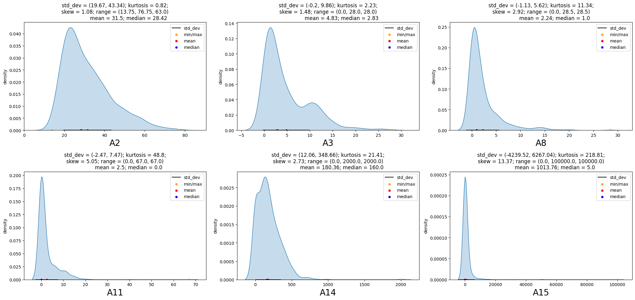
Univariate Analysis - Continous Variables

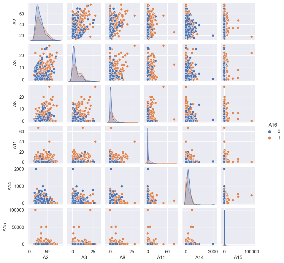
Findings from the distribution of numeric variables at overall level and considering the application status are as below:

• The dispersion/standard deviation of numeric variables for the applications granted credit extends over a wide range.
• The shape of distribution is similar in both groups for the variables ‘A2’, ‘A3’ and ‘A14’.
• In particular, Numeric variables ‘A11’ and ‘A15’ is concentrated to a very narrow range for the applications not granted credit.

eda_overview.UVA_numeric(data = df2, var_group = contAttr)

# Apply the default theme
sns.set_theme()
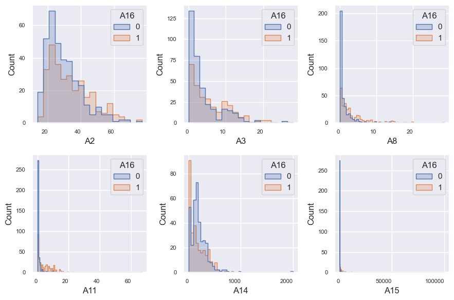
t = eda_overview.UVA_numeric_classwise(df2, 'A16', ['A16'],
                                       colcount = 3, colwidth = 3,
                                       rowheight = 3,
                                       plot_type = 'histogram', element = 'step')

plt.gcf().savefig(path+'Numeric_interaction_class.png', dpi = 150)

t = eda_overview.distribution_comparison(df2, 'A16',['A16'])[0]
t

Value	Maximum		Minimum		Range		Standard Deviation		Unique Value count
A16 category	0	1	0	1	0	1	0	1	0	1
Continous Attributes
A2	74.830	76.75	15.17	13.75	59.660	63.0	10.7192	12.6894	222	219
A3	26.335	28.00	0.00	0.00	26.335	28.0	4.3931	5.4927	146	146
A8	13.875	28.50	0.00	0.00	13.875	28.5	2.0293	4.1674	67	117
A11	20.000	67.00	0.00	0.00	20.000	67.0	1.9584	6.3981	12	23
A14	2000.000	840.00	0.00	0.00	2000.000	840.0	172.0580	162.5435	100	108
A15	5552.000	100000.00	0.00	0.00	5552.000	100000.0	632.7817	7660.9492	110	145

t.to_csv(path +'NumericDistributionComparison.csv')

# Inspecting number of unique values
df2[contAttr].nunique()

A2     340
A3     213
A8     131
A11     23
A14    164
A15    229
dtype: int64

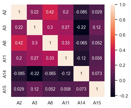
Bivariate Analysis - Continous Variables

Findings from the correlation plot are as below :

• No significant correlation between any pair of the features
• No significant correlation between any pair of feature and target

# Continous Variables are A2, A3, A11, A14, A15
contAttr = ['A2', 'A3','A8', 'A11', 'A14', 'A15']

# Target Variable is A16
targetAttr = ['A16']

df2[contAttr+targetAttr]

	A2	A3	A8	A11	A14	A15	A16
0	30.83	0.000	1.25	1.0	202.0	0.0	1
1	58.67	4.460	3.04	6.0	43.0	560.0	1
2	24.50	0.500	1.50	0.0	280.0	824.0	1
3	27.83	1.540	3.75	5.0	100.0	3.0	1
4	20.17	5.625	1.71	0.0	120.0	0.0	1
...	...	...	...	...	...	...	...
685	21.08	10.085	1.25	0.0	260.0	0.0	0
686	22.67	0.750	2.00	2.0	200.0	394.0	0
687	25.25	13.500	2.00	1.0	200.0	1.0	0
688	17.92	0.205	0.04	0.0	280.0	750.0	0
689	35.00	3.375	8.29	0.0	0.0	0.0	0

653 rows × 7 columns

# Bivariate analysis at overall level

plt.rcdefaults()
#sns.set('notebook')
#sns.set_theme(style = 'whitegrid')
sns.set_context(font_scale = 0.6)
from pandas.plotting import scatter_matrix
scatter_matrix(df2[contAttr+targetAttr], figsize = (12,8));

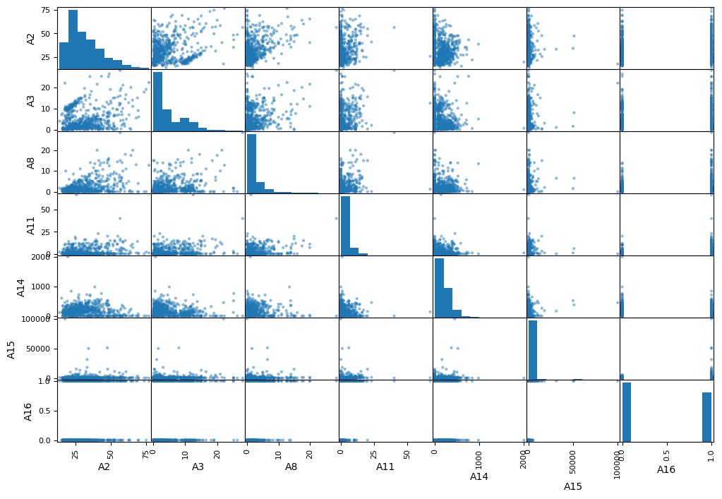
# Bivariate analysis taking into account the target categories

#sns.set('notebook')
sns.set_theme(style="darkgrid")
sns.pairplot(df2[contAttr+targetAttr],hue= 'A16',height = 1.5)

<seaborn.axisgrid.PairGrid at 0x7fc08ae9e790>

df2[contAttr+targetAttr].dtypes

A2     float64
A3     float64
A8     float64
A11    float64
A14    float64
A15    float64
A16      int64
dtype: object

# Correlation table
df2[contAttr].corr()

	A2	A3	A8	A11	A14	A15
A2	1.0000	0.2177	0.4176	0.1982	-0.0846	0.0291
A3	0.2177	1.0000	0.3006	0.2698	-0.2171	0.1198
A8	0.4176	0.3006	1.0000	0.3273	-0.0648	0.0522
A11	0.1982	0.2698	0.3273	1.0000	-0.1161	0.0584
A14	-0.0846	-0.2171	-0.0648	-0.1161	1.0000	0.0734
A15	0.0291	0.1198	0.0522	0.0584	0.0734	1.0000

# Heatmap for correlation of numeric attributes
fig, ax = plt.subplots(figsize=(5,4))
sns.heatmap(df2[contAttr].corr(), annot = True, ax = ax, annot_kws={"fontsize":10});

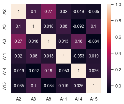
# Correlation matrix for customers not granted credit
fig, ax = plt.subplots(figsize=(5,4))
sns.heatmap(df2[df2['A16'] == 0][contAttr].corr(), ax = ax, annot_kws={"fontsize":10}, annot = True);

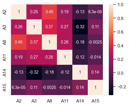
# Correlation matrix for customers granted credit
fig, ax = plt.subplots(figsize=(5,4))
sns.heatmap(df2[df2['A16'] == 1][contAttr].corr(),ax = ax,
            annot_kws={"fontsize":10}, annot = True);

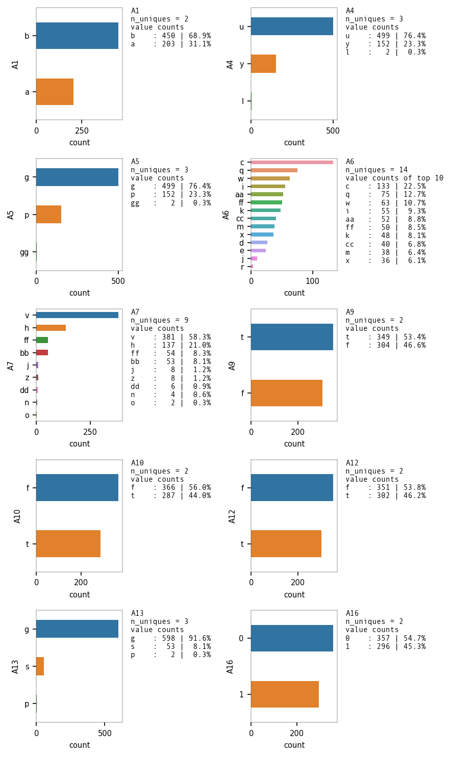
Univariate Analysis - Categorical Variables

# Continous Variables are A2, A3, A8, A11, A14, A15
# Categorical Input Variables are A1, A4, A5, A6, A7, A9, A10, A12, A13
# Target Variable is A16 and is categorical.

catAttr = ["A1","A4", "A5", "A6", "A7", "A9", "A10", "A12", "A13"]

eda_overview.UVA_category(df2, var_group = catAttr + targetAttr,
                          colwidth = 3,
                          rowheight = 2,
                          colcount = 2,
                          spine_linewidth = 0.2,
                          nspaces = 4, ncountspaces = 3,
                          axlabel_fntsize = 7,
                          ax_xticklabel_fntsize = 7,
                          ax_yticklabel_fntsize = 7,
                          change_ratio = 0.6,
                          infofntsize = 7)

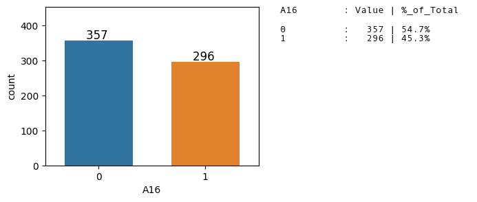
Distribution of the Target Class

Dataset is balanced as the ratio of the binary classes is ~55:45.
We can use Accuracy as a Evaluation metric for the classifier model.

plt.figure(figsize = (4,3), dpi = 100)
ax = sns.countplot(x = 'A16', data = df2, )
ax.set_ylim(0, 1.1*ax.get_ylim()[1])

axes_utils.Add_data_labels(ax.patches)
axes_utils.Change_barWidth(ax.patches, 0.8)
axes_utils.Add_valuecountsinfo(ax, 'A16',df2)

Continued on

Next page
Classic Jupyter notebook