A New Generalized Weighted Weibull Distribution

In this post, we will use R to plot generalized Weighted Weibull Distribution by varying the parameters alpha,lambda and gamma.

For the theory, We have referred to the paper “A New Generalized Weighted Weibull Distribution” by Salman Abbas, Gamze Ozal, Saman Hanif Shahbaz and Muhammad Qaiser Shahbaz. Check the link

Abstract

In this article, we present a new generalization of weighted Weibull distribution using Topp Leone family of distributions. We have studied some statistical properties of the proposed distribution including quantile function, moment generating function, probability generating function, raw moments, incomplete moments, probability, weighted moments, Rayeni and q−th entropy. We have obtained numerical values of the various measures to see the effect of model parameters. Distribution of order statistics for the proposed model has also been obtained. The estimation of the model parameters has been done by using maximum likelihood method. The effectiveness of proposed model is analyzed by means of a real data sets. Finally, some concluding remarks are given.

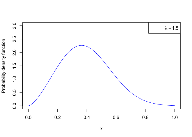
Probability Density Function

The formula for pdf

f(x) = (1+λ^γ)αγx^γ − 1e^{−α**x^γ(1+λ^γ)}

# Probability Density Function
x <- seq(0,1, length = 1000)
pdfx <- function(x, lambda = 1, alpha = 1, gamma = 2)
  {
  (1+lambda^gamma)*alpha*gamma*x^(gamma-1)*exp(-1*alpha*x^gamma*(1+lambda^gamma))
}

lamda = c(1.5)

plot(x,pdfx(x, alpha = 2, gamma = 2.5, lambda = 1.5),
     type = 'l', col = 'blue',
     ylim = c(0,3), ylab = "Probability density function")
legend("topright",lwd=1, cex = 1, col = c("blue"),
       legend = c(expression(lambda == paste('1.5'))))

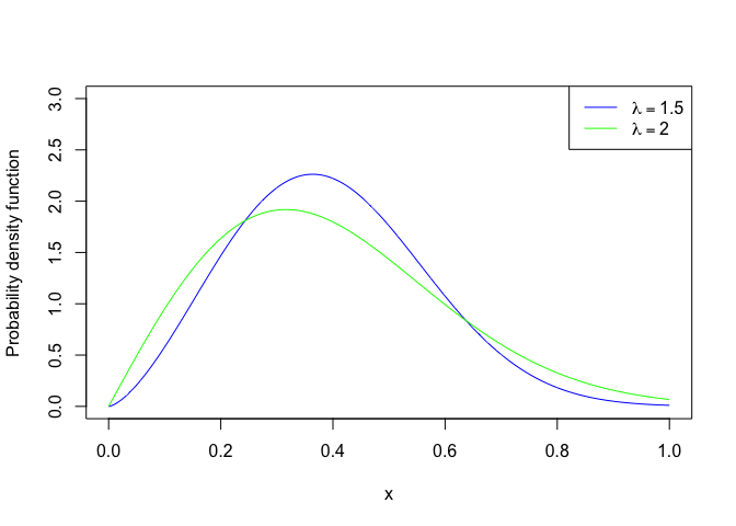
# Probability Density Function
x <- seq(0,1, length = 1000)
pdfx <- function(x, lambda = 1, alpha = 1, gamma = 2)
  {
  (1+lambda^gamma)*alpha*gamma*x^(gamma-1)*exp(-1*alpha*x^gamma*(1+lambda^gamma))
}

plot(x,pdfx(x, alpha = 2, gamma = 2.5, lambda = 1.5),
     type = 'l', col = 'blue',
     ylim = c(0,3), ylab = "Probability density function")
lines(x,pdfx(x, lambda = 2), type = 'l', col = 'green')

legend("topright",lwd=1, cex = 1, col = c("blue", 'green'),
       legend = c(expression(lambda == paste('1.5')),  
                  expression(lambda == paste('2'))))

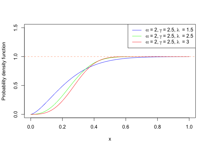
Cumulative Density Function

The formula for cdf

F(x) = 1 − e^{−α**x^γ(1+λ^γ)}
for x, α, λ > 0

Legend Creation

We have used bquote and as.expression are powerful tools for annotating figures with mathematical notation in R.

bquote(““~ alpha == 2,lambda == 1.5~”“)
as.expression(bquote(”“~alpha == 2, gamma == 2.5, lambda == 1.5~”“))

expression in R

Highly recommended links on expressions :

expression returns a vector of type “expression” containing its arguments (unevaluated).
expression and is.expression are primitive functions.
expression is ‘special’: it does not evaluate its arguments.

par_labels1 = c(expression(alpha ~“= 2,”~ gamma~“= 2.5,”~lambda~” = 1.5”))
par_labels1
eval(par_labels1)

R code and plot

#Cumulative Density Function
x <- seq(0,1, length = 1000)
cdfx <- function(x, lambda = 1, alpha = 1, gamma = 2)
  {
  1-exp(-1*alpha*x^lambda*(1+lambda^gamma))
}

par_labels1 = c(expression(alpha ~"= 2,"~ gamma~"= 2.5,"~lambda~" = 1.5"))
par_labels2 = c(expression(alpha ~"= 2,"~ gamma~"= 2.5,"~lambda~" = 2.5"))
par_labels3 = c(expression(alpha ~"= 2,"~ gamma~"= 2.5,"~lambda~" = 3"))
#parlabels = rbind(par_labels1,par_labels2, par_labels3)

plot(x,cdfx(x, alpha = 2, gamma = 2.5, lambda = 1.5),
     type = 'l', col = 'blue',
     ylim = c(0,1.5), ylab = "Probability density function")

lines(x,cdfx(x, alpha = 2, gamma = 2.5, lambda = 2.5), type = 'l', col = 'green' )
lines(x,cdfx(x, alpha = 2, gamma = 2.5, lambda = 3), type = 'l', col = 'red' )

legend("topright",lwd=1, cex = 1, col = c("blue", "green","red"),
       legend = c(par_labels1, par_labels2, par_labels3))

abline(h = 1, col = "lightsalmon", lty = 2)

** Note : This file was originally in Rmarkdown format and converted into rgular markdown. Know more : https://bookdown.org/yihui/rmarkdown/markdown-document.html

Bhaskar J Roy